APPENDIX C Paper on Zhao's Modified Cosmological Model

Peter Zhao

Taizhou Research Institute, Zhejiang University, China

The inflation-based Lambda Cold Dark Matter cosmological model has been accepted as the standard model of big bang cosmology. The success of the model lies with its ability of explaining the clear structure in the power spectra of the cosmic microwave background. The parameters inferred from the power spectra can predict light-element abundances based on big bang nucleosynthesis, and the observed abundances are in good agreement with the predicted values except for the ⁷Li abundance. More seriously, the inferred Hubble constant H~0~ = 67.4±0.5 kms^-1Mpc^-1 is significantly lower than the value (74.03±1.42 kms^-1Mpc^-1) measured locally from 70 long-period Cepheids in the Large Magellanic Cloud (LMC). Here, we show that all the discrepancies can be naturally resolved if we assume that the cold dark matter is the antimatter with negative mass, and that the universe has a fixed center close to the earth. The earth-center universe agrees with consistent observations of the quantized red shift.

The inflation-based Lambda Cold Dark Matter (ΛCDM) cosmological model assumes that the universe contains three major components: dark energy, cold dark matter, and ordinary matter. The model contains seven adjustable parameters and can well explain the clear structure in the power spectra of the cosmic microwave background (CMB). Based on the inferred parameters from the CMB spectra, the cosmologists can quantitatively explain the observed primordial abundances of light-elements such as ⁴He, deuterium, and ³He. Because of its simplicity and reasonable success in explaining the most cosmic properties, it has been called the standard model of big bang cosmology.

On the other hand, there are some important drawbacks in the model. First, the observed primordial ⁷Li abundance is about a factor of 2-3 smaller than the predicted value [1]. Second, the Hubble constant H~0~ = 67.4±0.5 kms^-1Mpc^-1 inferred from the CBM power spectra [2] is much lower than that (74.03±1.42 kms^-1Mpc^-1) measured locally from 70 long-period Cepheids in the Large Magellanic Cloud (LMC) [3]. Third, the model assumes asymmetry of matter and antimatter, which is inconsistent with the standard model of particle physics.

Here, we show that these discrepancies can be naturally resolved if we assume that the cold dark matter has negative mass, and the universe has a fixed center close to the earth. The negative mass of the cold dark matter (the cold antimatter) provides a gravitational red shift, which is also proportional to the distance r from us if the total matter density $\rho_{m}$(r) at present is proportional to 1/r at sufficiently large r. Then, the locally measured Hubble constant H~loc~ is the sum of H~0~ due to the expansion of the universe and H~g~ due to the gravitational red shift. The assumption of the earth-center universe agrees with frequent observations of the quantized red shift [4].

We are quite familiar with positive mass, but the concept of negative mass is quite exotic. We know that a positive mass gravitationally attracts all surrounding positive masses. However, a negative mass gravitationally repels all surrounding positive masses. The situation here is just opposite to the electrostatic interaction between charged particles: like charges repel each other while unlike charges attract each other. For a positive-negative mass particle pair, the net mass of the pair is equal to zero if both masses have the same magnitude. They will repel each other and undergo a runaway motion.

In our current model, the matter density $\rho_{m}$(r) at present is assumed to be $\rho_{0}$for r < a and $\rho_{m}$(r) = ${a\rho}_{0}/r$ for r$\geq a$ (where a is a finite radius). The boundary of the current universe comprises the cold matter and anti-baryons to keep the symmetry of matter and antimatter. The matter and antimatter in the boundary do not produce any gravity in the interior of the universe according to the gravitational Gauss' law (by analogy to the electric Gauss' law), so the ΛCDM cosmological model is still valid for the interior of the universe. The boundary of the universe should expand with a speed close to the speed of light c. Then the radius R~0~ of the present universe is approximately equal to ct~0~, where t~0~ is the age of the universe.

We now use the gravitational Gauss' law to determine the gravitational field in the interior of the universe. When the negatively massed cold dark matter dominates over the positively massed baryons, the gravitational field $\overrightarrow{g}(r)$ points radially outward. The light traveling towards the center will undergo a red shift in such a gravitational field according to the Einstein theory of general relativity:

Applying the Gauss' law in the region of $r > a$ yields,

where

$ = 2\pi a\rho_{0}r^{{2} - \frac{2\pi}{3}a}{3}\rho_{0}$.

Then

The total mass in the interior of the universe can be expressed as $\frac{4}{3}\pi R_{0}^{3}\rho_{m}$, where $\rho_{m}$ is the average matter density. The total mass is also given by

Then

$ 2\pi a\rho_{0}R_{0}^{{2} - \frac{2\pi}{3}a}{3}\rho_{0} = \frac{4}{3} \pi R_{0}^{3}\rho_{m}$. (4)

Using the fact that R~0~ $\gg $a, we obtain \rho_{0} = \frac{2R_{0}}{3a}\rho_{m}.

Finally, we obtain the magnitude of the gravitational field for r > a:

Substituting Eq. 5 into Eq. 1, we have

where

Then

For r >> a, H_{g} = \frac{4\pi G{\rho_{m}R}_{0}}{3c}. \

Therefore

Now we apply the Gauss' law to the region of $r < a$:

then

where $B = 8\pi G{\rho_{m}t}_{0}/9a.$

In the ΛCDM cosmological model, the expansion of the universe is parametrized by a dimensionless scale factor a = a(t) with t counted from the birth of the universe. At present, a~0~ = a(t~0~) =1. The expansion rate is described by the time-dependent Hubble parameter H(t), defined as H(t) = da/(adt). The first Friedmann equation is used to describe the expansion of the universe, and this equation can be conveniently written in terms of various density parameters as:

$ H(a) = H_{0}\sqrt{{(\Omega}_{b} + \Omega_{c})a^{{- 3}{+ \Omega}_{rad}a}{- 4}{+ \Omega}_{k}a^{{- 2}{+ \Omega}_{DE}a}{- 3(1 + w)}}$,

where the present-day density parameter $\Omega_{x}$ for various species is defined as the dimensionless ratio:

where the subscript x is: b for baryons, c for cold dark matter, rad for radiation, and DE for dark energy. In the minimal six-parameter model with $w = - 1$, ${\Omega_{k} = 0, and \Omega}_{rad}\sim 0,$ Friedmann equation is simplified as

$ H(a) = H_{0}\sqrt{{(\Omega}_{b} + \Omega_{c})a^{- 3}{+ \Omega}_{DE}}$ (9)

with $\Omega_{m} + \Omega_{DE}$ = 1 and $\Omega_{m}$ = $\Omega_{b} + \Omega_{c}$. The equation has an analytic solution

In the above equations, $\Omega_{b}$, $\Omega_{c},$and $\Omega_{DE}$ are all positive numbers because only matter with positive mass is considered in the Friedmann equation. However, when the cold dark matter with negative mass is considered, the space is filled with both matter and antimatter, we need to consider the sign of each component. If the matter dominates over the antimatter, the net matter density is still positive and the net gravitational interaction is attractive. This naturally ensures that the first term $8\pi G\rho/3$ of the Friedmann equation is a positive number. On the other hand, if the antimatter dominates over the matter, the net matter density is negative, but the net gravitational interaction is still attractive. To agree with the Friedmann equation, we still keep the positive signs of $\Omega_{c},{ \Omega}_{b}$, and $\Omega_{DE}$ (absolute values) but replace ${\Omega_{m} = \Omega}_{c} + \Omega_{b}$in the matter-dominated case with ${\Omega_{m} = \Omega}_{c} - \Omega_{b}$ in the antimatter-dominated case.

Now we consider the CMB experiments that reveal sound waves in the fine angular structure of the temperature anisotropies. The power spectrum of the temperature maps exhibits clear peaks, which are closely related to the acoustic phenomena of the universe. A simple way to understand this phenomenon is to consider that the universe was a photon-baryon plasma (fluid) when its temperature was above 3,000 K. The photon-baryon fluid is sitting in the gravitational potential wells that are the seeds of structure in the universe. As gravity tries to compress the fluid, the radiation pressure resists, which leads to acoustic oscillations. The system is equivalent to a baryon mass on a spring falling under gravity. Compression occurs in the gravitational potential wells while rarefaction in the hills. Sound waves stop oscillating at recombination when the baryons release the photons. The acoustic modes at extrema of their oscillations become the peaks in the CMB power spectrum by recombination. The first peak represents the mode that the compressed one inside potential well before recombination, the second peak corresponds to the mode that compressed and then rarefied, and so on. Amplitudes of the odd-number peaks are higher than those of even-number peaks because the mass loading of baryons makes the oscillation asymmetric: the extrema that represent compressions inside the wells are enhanced over those that represent rarefactions in the hills.

At the early universe, quantum fluctuations may generate both density enhancements and deficits. When the matter dominates over the antimatter in the space (the net matter density is positive), the gravitational potential hills appear in regions of deficits and the potential wells in regions of enhancements. This is because a baryon gravitationally attracts the surrounding matter with a net mass of the positive sign. In contrast, when the antimatter dominates over the matter in the space (the net matter density is negative), the gravitational potential hills appear in regions of enhancements and the potential wells in regions of deficits. This is because a baryon gravitationally repels the surrounding matter with a net mass of the negative sign.

The above simple picture tells us that the gravitational potential landscapes (containing plane waves of various wavelengths) in both cases are the same. This implies that the CMB spectra in both cases are identical if $\Omega_{b}$, $\Omega_{m},$ $\Omega_{DE}$, and H~0~ are identical. Therefore, the parameters inferred from the CMB spectra are equally applicable to the current case where the antimatter dominates over the matter.

In two equations (Eq. 7 and Eq. 10), there are three unknown variables: $H_{0}$, $\Omega_{m},$ and $t_{0}$. In order to find the solutions of $H_{0}$, $\Omega_{m},$ and $t_{0}$, we need a third equation related to these variables. Fortunately, W. J. Percival et al. found an important constraint on the flat cosmologies from CMB power spectra [5]. They showed that $\Omega_{m}h^{{3.4} =$ constant independent of other parameters, where ${h = H}_{0}$/(100 kms}-1^Mpc-1^{). From the CMB spectra before 2002, they obtained $\Omega_{m}h}{3.4}$= $0.081 \pm 0.012$. From more accurate CMB spectra of 2018 Planck final mission [2], we find that

$ \Omega_{m}h^{3.4} = 0.08241 \pm 0.00046$ (11)

It is apparent that the values of $\Omega_{m}h^{{3.4}$inferred from the previous and current CMR spectra are the same within the uncertainties. With $H_{loc}$= 74.03±1.42 kms}-1^Mpc-1^{, we can solve Eq. 7, Eq. 10, and the equation: $\Omega_{m}h}{3.4} = 0.08241$ to find the solutions of $H_{0}$, $\Omega_{m},$ and $t_{0}$. Our solutions are the following: t~0~ = 13.8157±0.0021 Gyr, $\Omega_{m}$ = ${0.400}_{- 0.039}^{{+ 0.043}$, and $H_{0}$ = ${62.838}_{- 1.858}}{+ 1.922}$ kms^-1Mpc^-1.

W. J. Percival et al. also showed that $\Omega_{b}h^{{2}$ depends on $h$. The contour of $\Omega_{b}h}{2}$ vs $h$ corresponding to the maximum likelihood of 2.3 is replotted in Figure C1. From Figure C1 and the inferred $H_{0}$, we obtain $\Omega_{b}h^{{2}$= 0.0198±0.0005 and the ratio of the baryon density to the photon density $\eta_{10} = 5.55 \pm 0.13$. From the calculated light element abundances based on the big-bang nucleosynthesis (BBN) model [6] and $\Omega_{b}h}{2}$= 0.0198±0.0005, we find the following primordial abundances: ⁷Li/H = (3.90$\pm 1.50) \times 10^{{- 10},$ D/H = (3.17$\pm 0.77) \times 10}{- 5}$, ⁴$He/H = 0.2474 \pm 0.0002$, and ³He/H = (1.10$\pm 0.19) \times 10^{- 5}$.

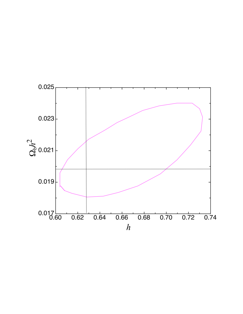
Figure C1: The contour of $\Omega_{b}h^{2}$ vs $h$, which corresponds to the maximum likelihood of 2.3. The figure is replotted from figure 2 of Ref. 5.

Different groups have measured Li/H abundances and the results are summarized in Figure C2. The predicted ⁷Li/H abundance is in the range of (2.61-4.49)$\times 10^{{- 10}$ while the measured abundance is in the range of (1.34-3.23)$\times 10}{- 10}$. A simple averaging for the five data points yields ⁷Li/H = (2.18$\pm 0.07) \times 10^{{- 10}.$The predicted lower limit of 2.40$\times 10}{- 10}$ is close to the average value within the standard deviation. Therefore, the lower limit of the $\Omega_{b}h^{2}$parameter is in reasonable agreement with the measured Li/H abundance.

There are two consistent data [12,13] for the primordial ⁴$He/H$ abundance: $0.2449 \pm 0.0040$ and $0.2446 \pm 0.0029$. Both data agree with the predicted value of $0.2474 \pm 0.0002$ within the experimental uncertainties.

The measured deuterium abundance D/H is 2.50$\pm 0.5 \times 10^{{- 5}$ (Ref. 14), which is within the predicted range: (3.17$\pm 0.77) \times 10}{- 5}$. The measured ³He/H =1.5$\pm 0.2 \times 10^{{- 5}$ (Ref. 15). The lower limit of the measured value is very close to the predicted upper limit of 1.29$\times 10}{- 5}$. Therefore, the lower limit of the $\Omega_{b}h^{{2}$parameter is in good agreement with the measured value of the} 3^He abundance.

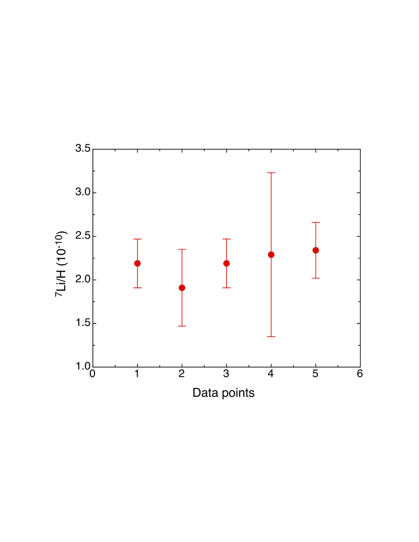
Figure C2: The measured ⁷Li/H abundances from different groups. The data points are taken from Refs. [7-11].

If we use the lower limit of $H_{loc}$ = 72.6 kms^-1Mpc^-1 and the lower limit of $\Omega_{m}h^{{3.4}$= 0.08195, we find *t*~0~ = 13.8398 billion years, $\Omega_{m}$ = 0.440, and $H_{0}$ = 61.0 kms}-1^Mpc-1^{. These parameters lead to the lowest value of $\Omega_{b}h}{2}$= 0.0193. This value predicts the lowest deuterium abundance of 2.40$\times 10^{{- 5}$, the highest} 3^{He abundance of 1.29$\times 10}{- 5}$, and the lowest ⁷Li abundance of 2.61$\times 10^{{- 10}$. All these predicted values are consistent with the observed ones within the experimental uncertainties. Therefore, the CMB spectra and the observed light-element abundances narrow down the parameters: $H_{loc}$ = 72.6 kms}-1^Mpc-1^{, $H_{0}$ = 61.0 kms}-1^Mpc-1^{, $\Omega_{b}h}{2}$= 0.0193, $\Omega_{m}$ = 0.440, and t~0~ = 13.8398 billion years. It is remarkable that t~0~ = 13.8398 billion years, which is very close to 7¹² years. The difference between 13.8398 billion years and 7¹² years is only 0.011%.

We now turn to the red shift data at distances below Virgo Cluster (Figure C3), which are taken from Figure 1.3 of Ref. 16 and Figure 1 of Ref. [17]. The best linear fit to the data yields $H_{loc}$ = 67.48$\pm 2.70$kms^-1Mpc^-1. This number is consistent with H~0~ = 67.4±0.5 kms^-1Mpc^-1 inferred from the CMB data but disagrees with the value (74.03±1.42 kms^-1Mpc^-1) measured locally from 70 long-period Cepheids in the Large Magellanic Cloud. The solid black line in Figure C3 is the best fitted curve by Eq. 8 with the fixed parameters inferred from $H_{loc}$ = 72.6 kms^-1Mpc^-1 and $\Omega_{m}h^{3.4}$= 0.08195 and a fitting parameter a. The fitting parameter a is found to be 12.31$\pm 3.87$ Mpc. Therefore, our model can naturally resolve the discrepancy.

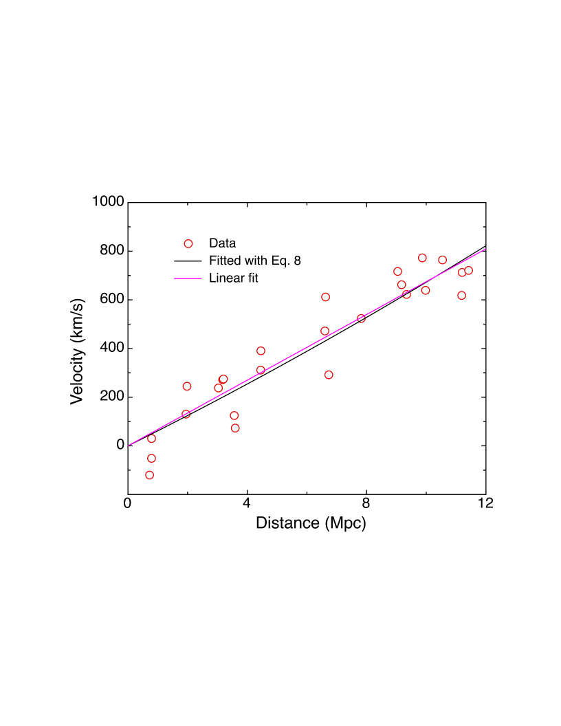
Figure C3: Red shift velocities at the distances below Virgo Cluster. The data are taken from Figure 1.3 of Ref. 16 and Figure 1 of Ref. [17].

For r > a, our model agrees with the red shift data at larger distances (>15 Mpc) compilated by the Hubble Space Telescope Key Project that finalized in 2001 (see Ref. 17). In Figure C4, we plot the data at the distances between 15-392 Mpc. The open green squares represent the calculated values of Eq. 6 with the fixed parameters inferred from $H_{loc}$ = 72.6 kms^-1Mpc^-1 and $\Omega_{m}h^{3.4}$= 0.08195 and the fixed parameter a = 12.31 Mpc. The calculated points have no adjustable parameter.

We can also fit the data by a linear equation: red-shift velocity = $H_{loc}$d, where d is the distance from us. The best liner fit to the data yields $H_{loc}$ = 72.71±0.79 kms^-1Mpc^-1 (see solid black line). The differences between the calculated values of Eq. 6 and the best linearly fitted curve are negligibly small. If we fit the data by Eq. 6 with one free parameter H~0,~ we obtain H~0~ = 61.14±0.79 kms^-1Mpc^-1, which is very close to the value of 61.0 kms^-1Mpc^-1 inferred from $H_{loc}$ = 72.6 kms^-1Mpc^-1 and $\Omega_{m}h^{3.4}$= 0.08195.

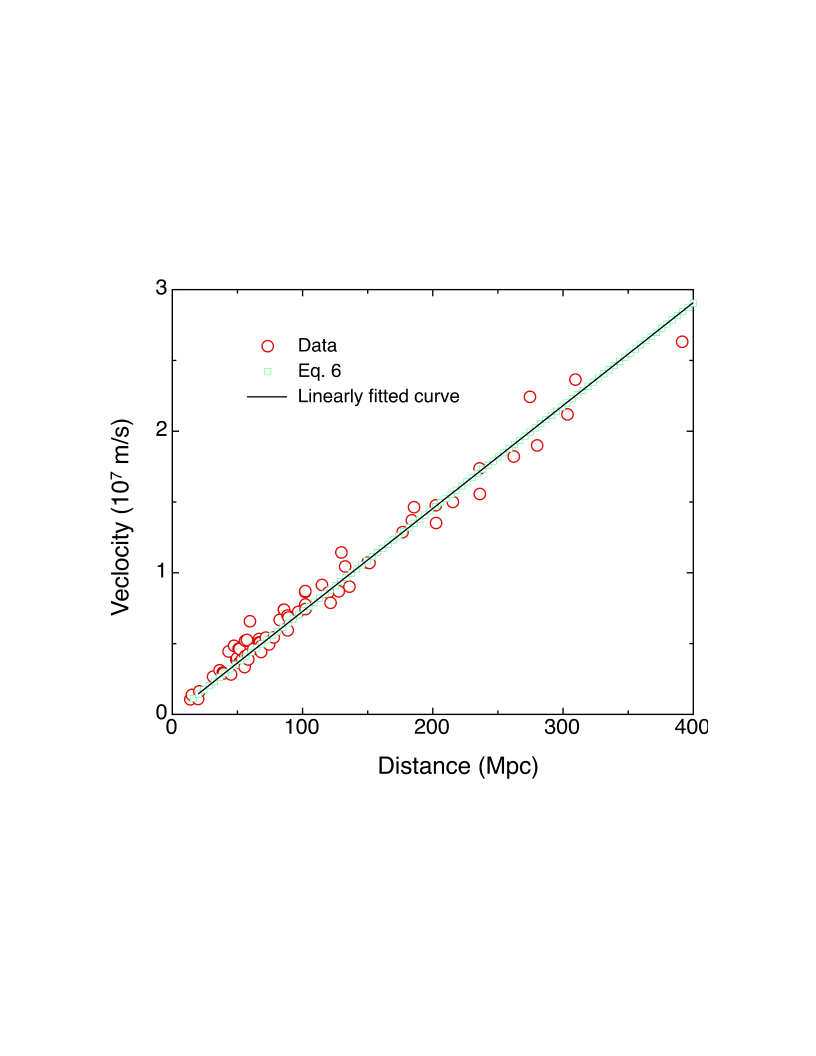
Figure C4: Red-shift velocities at large distances. These data were compilated by the Hubble Space Telescope Key Project that finalized in 2001 [17]. The open green squares represent the calculated values of Eq. 6 with the fixed parameters inferred from $H_{loc}$ = 72.6 kms^-1Mpc^-1 and $\Omega_{m}h^{{3.4}$= 0.08195 and the fixed parameter *a* = 12.31 Mpc. The best linear fit to the data yields $H_{loc}$ = 72.71±0.79 kms}-1^Mpc-1^ (solid black line).

In conclusion, our modified ΛCDM cosmological model almost perfectly resolves all the discrepancies between the model and the observed cosmic properties. The negative mass of the cold dark matter and the earth-centered universe are the essential components in the modified model. The age of our universe is almost exactly equal to 7¹² years if we assume that the speed of light is a constant and the theory of general relativity is valid.

[1] R. H. Cyburt, B. D. Fields, and K. A. Olive, JCAP 11, 012 (2008).

[2] Planck 2018 results. VI. Cosmological parameters, arXiv:1807.06209v1 [astro-ph.CO],

17 June 2018.

[3] A. G. Riess et al., APJ 876, 85 (2019).

[4] D. R. Humphreys, TJ 16, 95 (2002); and references therein.

[5] W. J. Percival et al., MNRAS 337, 1068; arXiv:astro-ph/0206256v2, 22 Aug 2002.

[6] C. J. Copi, D. M. Schramm, and M. S. Turner, Science 267, 192 (1994).

[7] P. Bonifacio et al., Astron. Astrophys. 390, 91 (2002)

[8] L. Pasquini and P. Molaro, 1996 Astron. Astrophys. 307, 761 (1996).

[9] F. Thevenin et al., Astron. Astrophys. 373, 905 (2001).

[10] P. Bonifacio, Astron. Astrophys. 395, 515 (2002)

[11] J. Melendez and I. Ramirez, Astrophys. J. 615, L33 (2004).

[12] E. Aver, K. A. Olive, and E. D. Skillman, JCAP 2015, 011 (2015).

[13] A. Peimbert, M. Peimbert, and V. Luridiana, Rev. Mex. Astron. Astrofis. 52, 419,

(2016).

[14] F. Hersant, D. Gautier, and J. M. Hure, APJ 554, 391 (2001).

[15] J. Geiss and G. Gloeckler, Space Science Review 84, 239 (1998).

[16] W. C. Keel, The Road to Galaxy Formation (2nd ed. Springer, 2007 ), pp 7.

[17] W. Freeman et al., Astrophys. J 553, 47 (2001).